




A train has no differential.
Not “a simplified one”, not “one in the bogie” — none, anywhere. The two wheels of a wheelset are pressed onto one axle and turn at exactly the same rate forever. On a curve, where the outer wheel has further to go, that should be impossible.
What makes it possible is that the tread is not cylindrical. It is a cone, nominally 1 in 20, with the radius growing toward the flange. Shove the wheelset sideways and one wheel starts rolling on a bigger circle than the other, so the two ends of the axle advance at different rates and the wheelset yaws. That is the entire steering system of a railway vehicle: a taper, and the fact that the wheels are welded to the same shaft. No linkage, no actuator, nothing anybody adjusts.
Three things follow from it, and this piece is the three.
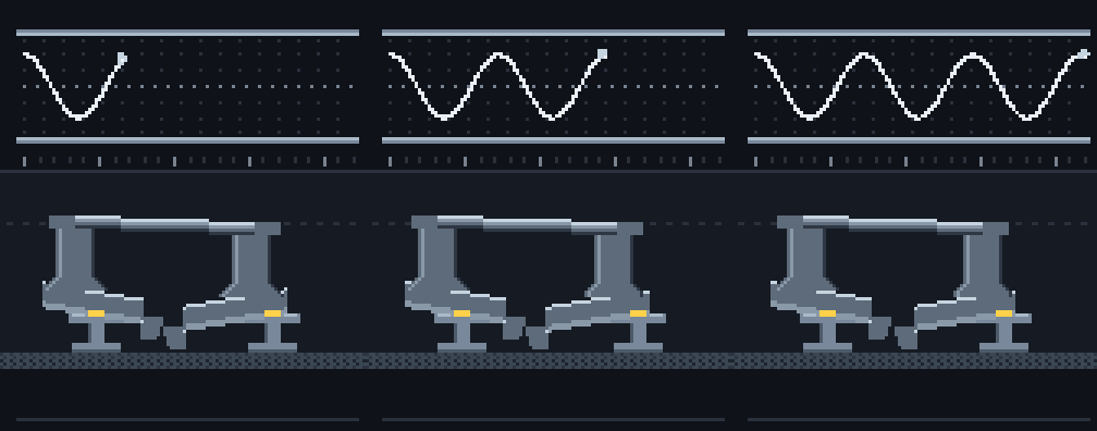
It weaves, and the weave has no clock in it
A displacement makes a radius difference, a radius difference makes a yaw, a yaw makes a displacement. That is a second-order system, and because every term in it is per-metre-of-track rather than per-second, the thing it produces is a wavelength:
lambda = 2*pi*sqrt(r0*b/taper)
       = 2*pi*sqrt(0.3556 * 0.7465 / 0.05)
       = 14.48 m
Klingel wrote that down in 1883 and there is no velocity in it. A wheelset
crossing a yard and one at line speed trace the same shape; they differ only
in how fast they trace it. The weave loop is the rolling constraint
integrated and nothing else, and validateGeometry() checks the trace’s zero
crossings against the closed form to half a percent — because if the integrator
and the formula ever disagreed, one of them would be describing a different
wheelset.
What that wavelength means in a vehicle is a frequency that happens to land exactly where people notice:
| speed | the weave arrives at |
|---|---|
| 30 km/h | 0.58 Hz |
| 50 km/h | 0.96 Hz |
| 144 km/h | 2.76 Hz |
It is tempting to go one step further and say that the sway you feel standing on a subway is this. That is not a claim this file can make: whether a given car’s lateral motion is kinematic hunting, bogie hunting or track geometry is a question about that car’s suspension. The honest statement is narrower and still worth having: the cone puts a weave into every wheelset on the railway at around 1 Hz at city speeds, for free, with no input at all.
It is unstable, and the cone is not what fixes it
Pure rolling conserves the weave: the weave loop runs 44 m and comes out at
the amplitude it went in at, and would do that forever. Real contacts do not
roll purely. They transmit force through creep — a small relative slip in a
contact patch the size of a coin — and once you put creep forces into the same
two equations, a free wheelset is unstable at every speed. Not above a
critical speed. Every speed.
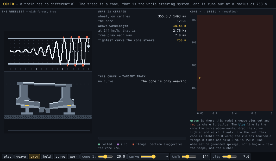
The grow loop is that: the same track, 144 km/h, a 0.3 mm nudge, and no
suspension. It builds through 150 m, reaches the flanges, and spends the rest
of its life banging between them — eight contacts in the frame.
The held loop is the same wheelset with a primary suspension attached, started hard against a rail at the full 7 mm, and
it comes back down a clean exponential — each swing about 2.6 times smaller
than the one before:
7.00 mm 2.67 1.02 0.39 0.15 0.06 …under a tenth of a millimetre by 30 m, with half the frame left over.
So the lesson a railway wheel teaches is the opposite of the one it looks like it teaches. The cone is a steering mechanism that cannot be left to itself. The thing that makes a train stable is the springs between the wheelset and the rest of the vehicle, and designing them is the whole subject.
It runs out at 758 metres
This is the part that surprises.
A curve of radius R needs the outer wheel to roll (R+b)/(R−b) times as far
as the inner one. The cone supplies radius difference at 2*taper*y, so the
sideways displacement a curve asks for is
y = b*r0/(taper*R)and a wheelset has about 7 mm of lateral play before a flange touches rail. Set those equal:
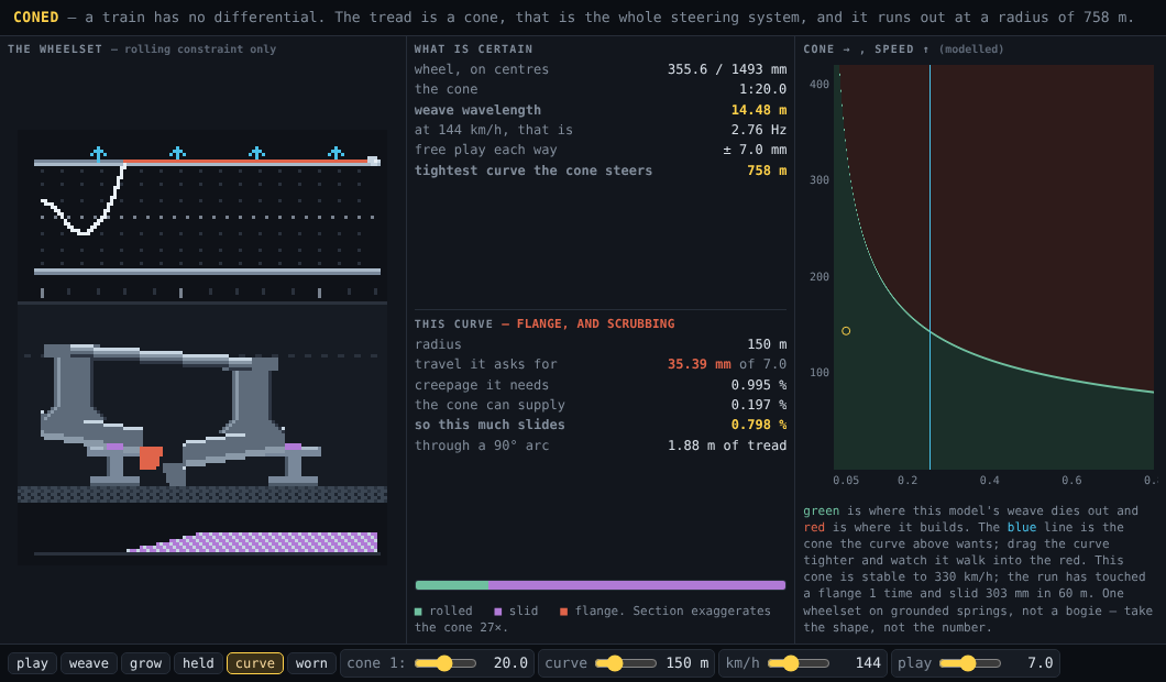
R* = b*r0/(taper * 7 mm) = 758 mSeven hundred and fifty-eight metres. That is the tightest curve a new 1:20 tread can steer on its own. A mainline curve is often tighter. A transit curve is tighter by a factor of five or ten. The whole elegant self-steering mechanism is in charge on tangent track and on the gentlest curves in the network, and essentially nowhere else.
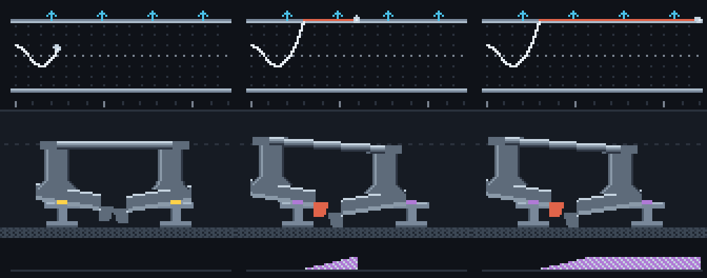
Run the curve loop — 150 m radius, which is an ordinary piece of subway — and
watch what it does instead. It weaves on the straight, enters the transition,
and goes to the flange and stays there:
| the cone is asked for | 35.39 mm |
| it has | 7.00 mm |
| creepage the curve needs | 0.995% |
| the cone can supply | 0.197% |
| so this slides | 0.798% |
0.798% of a 90° arc at 150 m radius is 1.88 metres of tread dragged sideways past rail, per wheelset, per curve. And it is not a near miss on adhesion either: the longitudinal force that creepage would need is 69.7 kN against a contact that can hold 14.7, so the demand is 4.7 times what friction will deliver. The contact is not creeping. It is sliding, grossly, which is the condition the literature puts behind curve squeal — the sound itself is a wheel’s acoustic modes and is not modelled here at all.
That is what the purple strip under the wheelset is counting.
And the fix costs you the top end
The obvious move is to grind a steeper cone, and it works exactly as advertised.
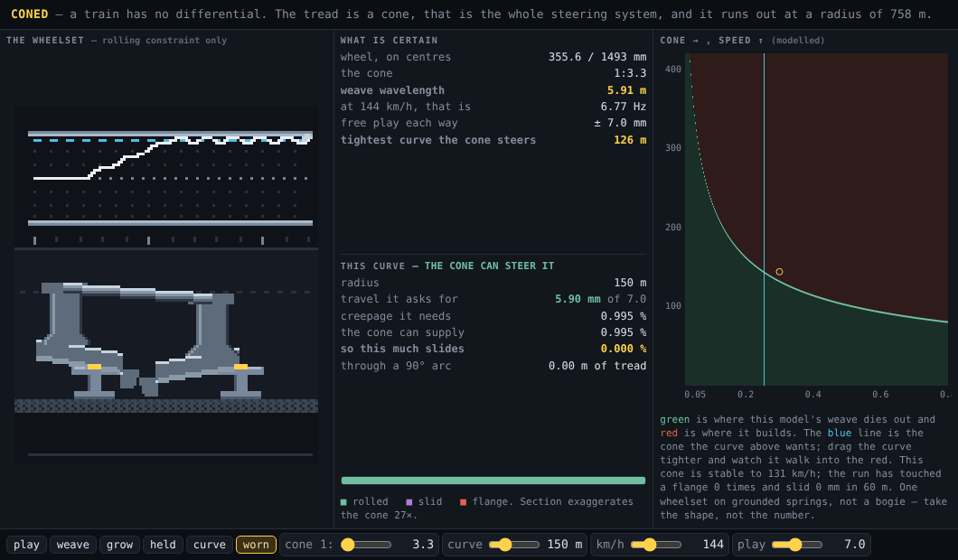
At an equivalent conicity of 0.30 — which is not exotic; it is roughly what
a worn wheel on a worn rail reaches once the contact climbs toward the flange
root — the same 150 m curve asks for 5.90 mm, which fits inside the play. The
worn loop steers it with 0.58 mm to spare and never touches a flange.
The bill arrives at the other end of the speed range. Conicity is the coupling term in the stability problem, so the same change that bought the curve takes the critical speed down with it:
| cone | tightest curve it steers | and the model’s critical speed |
|---|---|---|
| 1:40 | 1517 m | 481 km/h |
| 1:20 | 758 m | 330 km/h |
| 1:10 | 379 m | 230 km/h |
| 1:3.3 | 126 m | 131 km/h |
Which is the trade-off the whole subject is organised around, and it explains the two halves of the railway. A metro runs 150 m curves at 50 km/h, so it can afford all the conicity it likes and pays for the curves in metal — scrubbed treads, ground rail, squeal. A high-speed line cannot afford the conicity, so it buys the curves in civil engineering instead, and is built straight.
The demo’s right-hand panel is that sentence as a picture: the green region is where this model’s weave dies out, and the blue line is the cone the curve you have selected is demanding. Drag the curve tighter and watch the line walk into the red.
How far to trust this
Kept apart in the source and here, because they are not the same kind of claim.
Certain. All of the kinematics. The rolling radii, Klingel’s wavelength,
the displacement a curve demands, the radius at which that exceeds the play,
the creepage needed against the creepage available, and the sliding the
difference forces. Those are geometry and bookkeeping about a rigid wheelset on
rigid rails, and validateGeometry() asserts the ones this page leans on —
including the 758 m itself, so that if a constant ever drifts the build fails
instead of the prose quietly lying.
Modelled. Everything with a force in it. step() is the standard
two-degree-of-freedom wheelset — lateral and yaw — with linear creep
coefficients, a friction cap on each contact, a stiff one-sided flange stop, and
the primary suspension as springs to ground. It is not a bogie. A real vehicle
has two wheelsets in a frame with its own freedom to yaw, and its critical speed
is lower than anything in that table. Believe the signs and the shapes — free
wheelset grows, sprung wheelset decays, conicity buys curves and costs speed.
Do not quote the critical speed at anybody.
There is one more honest limit worth naming, because it decided how this file is organised. A wheelset on grounded springs does not curve properly. The lateral spring pulls it back toward the track centre, so its steady displacement in a curve is set partly by the spring instead of entirely by the cone: on a 2000 m curve where the geometry asks for 2.65 mm, the deliberately soft springs used here settle at 2.38, and a realistically stiff primary suspension settles at 0.20 — an order of magnitude short, steering almost not at all.
That is not a bug to patch. It is the reason the primary suspension is the central compromise in railway vehicle dynamics — the stiffness that holds the wheelset straight at speed is the stiffness that stops it turning — and here it is the reason the two curve loops run the rolling constraint, where the claims are geometry, while the two stability loops run the forces on tangent track, where springs to ground are a fair stand-in for a bogie going straight.
Where this sits
run-in is the same railway seen along its length — a mile of freight as a
chain with 5.21 m of slack in it — and treats each car as a point that follows
the track. This is what one of those points is actually doing underneath, and
the answer is that it is weaving at 14.48 m and, on anything tighter than a
third of a mile of radius, grinding.
The loops
- weave — tangent track, rolling constraint only. 14.48 m, forever, nowhere near a flange.
- grow — 144 km/h, creep forces, no suspension. 0.3 mm to flange contact in 150 m.
- held — the primary suspension in, started hard against a rail at 7 mm. 7.00, 2.67, 1.02, 0.39, and gone, over 60 m.
- curve — 10 m of tangent, a 20 m transition, then 150 m radius. It runs out of cone, sits on the outer flange, and the scrub strip fills.
- worn — the same curve at an equivalent conicity of 0.30. It steers it, inside the play, with nothing sliding.
Reading the frame
Three bands, and the middle one is drawn with its scales declared because they have to be:
- top — lateral displacement against distance down the track. The two rails are the flange limits; red is flange contact, purple is gross slip, and the blue arrows mean the displacement the curve wants is off the top of the chart.
- middle — the two contacts in section. Everything hangs off the one fixed thing, which is that the tread passes through the railhead crown, because the rail does not move. What the sideways travel changes is which part of the tread is over the rail — hence where the flange is, and how high that end of the axle rides. The axle bar has to stay straight: the two wheels are one forging and nothing is free to absorb the difference. The tread is drawn at 1:6 instead of 1:20 and sideways travel at 8×, so the rolling radius difference reads at about 27× life size; 1:20 across 135 mm of tread is a third of a pixel and there is no honest way to draw it small.
- bottom — how much is sliding, column by column, on the same distance axis.
Reuse
export/wheelset-<loop>-<n>.png— 1× frames (112×132). Render at integer scales with nearest-neighbour filtering.export/wheelset-sheet.png— every frame in one strip, in loop order.export/wheelset@4x.png— prescaled hero, the free wheelset at the flanges.
Source
No .aseprite — the canonical source is source/coned.mjs, which is the
kinematics, the dynamic model, the Routh test and the pixel drawing in one
file. Nothing is keyframed: a frame is renderFrame({ run, s }) evaluated at a
distance in metres down the track, and the wheelset is wherever the integration
put it. Regenerate everything with:
node source/render.mjs             # export/, media/ loops, thumb, demo copy
node scripts/screenshot-demo.mjs   # media/ demo shots, and the demo smoke test
(needs site/node_modules installed — the scripts resolve Chromium through
site/scripts/lib/chromium.mjs.)