Fanout

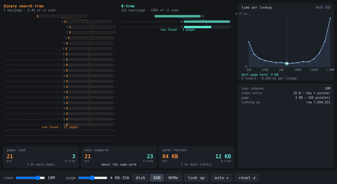
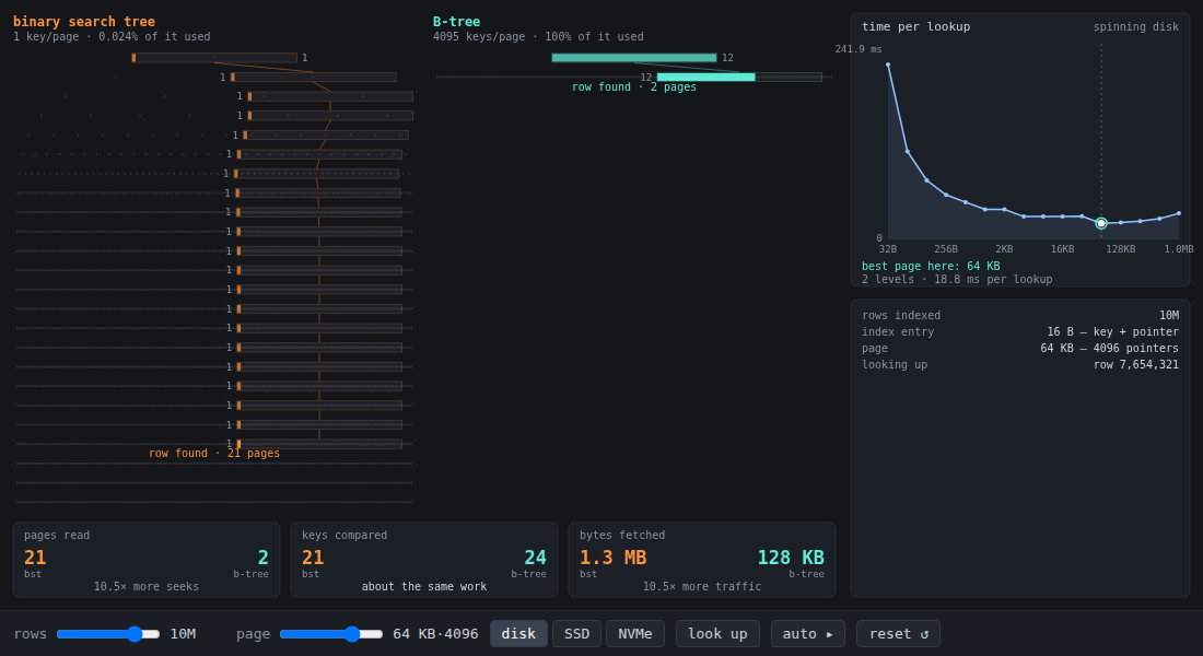
Ten million rows, one index entry each, and two ways to arrange them. On the left a binary search tree, one key per node. On the right a B-tree at whatever fanout the page size allows. Same rows, same lookup, both descending at once.

The usual way to sell a B-tree is “it’s shallower,” and the usual evidence is the descent: 21 page reads against 3. That is true and it is not the argument, because shallower would be worthless if the work per level went up to pay for it. So the piece counts three things instead of one.

Pages read: 21 against 3. The shape you expected.

Keys compared: 21 against 23. The B-tree does more comparison work. Each of its three pages holds up to 255 keys and you binary-search within the page — 8, 8 and 7 comparisons on the way down, against one per node twenty-one times. The card says “about the same work” because it is about the same work — the comparisons did not go anywhere, they just got repacked. Anyone who tells you a B-tree is asymptotically better at searching is describing a constant factor in a cost model that isn’t the one being billed.

Bytes fetched: 84 KB against 12 KB. Here is the cost model that is actually billed. Every box drawn on the path is one page, and both columns draw them the same width, because the device hands you a whole page either way. What differs is the fill. The B-tree’s pages are solid — 100% of each one gets used. The binary tree’s are a 3-pixel sliver in an empty frame: 16 bytes of key and pointer inside a 4096-byte page, 0.4% used, twenty-one separate times. The header over each column says the percentage out loud, and the slivers say it without words.

That is the whole thing. A B-tree is not a cleverer search. It is the same search, re-cut so that the unit of work matches the unit of purchase.

Two things that fall out

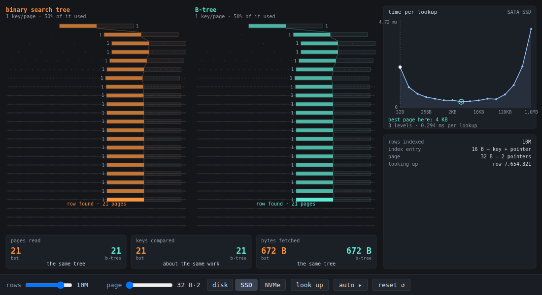
Set the page to 32 bytes and the B-tree becomes the binary search tree. Not approximately — the two columns go pixel-identical, 21 pages and 21 comparisons and 672 bytes each, and all three cards read the same tree. That is not a special case bolted on; search(n, 2, target) is the only search routine in src/fanout.js, and the left column is a call to it with fanout 2. A binary search tree is a B-tree whose pages are too small to be worth fetching. The fanout was never an algorithmic choice. It was a division: how many entries fit in whatever the hardware insists on handing you.

Which page size is best depends on the disk, and it moved. The curve on the right prices a lookup as one seek plus one page transfer per level, over every page size from 32 B to an absurd 1 MB. It has a floor in the middle, and the floor moves when you change the device:

• Spinning disk — 9 ms to find the sector, 160 MB/s once you’re there. Seeks dominate so completely that the answer is to buy depth down with enormous pages: the floor sits at 64 KB, two levels, 18.8 ms. Going from 32 B to 64 KB takes a lookup from 216 ms to 18.8 ms — an 11× swing decided entirely by how many entries you chose to put in a page.
• SATA SSD and NVMe — no sector to find, so transfer starts mattering and the floor climbs back down to 4 KB, three levels (0.29 ms and 0.03 ms).

Which is the mildly satisfying part: the 4 KB page is not a fossil we’re stuck with from the spinning-disk era. On flash it is roughly the right answer, and it’s the 64 KB answer that was the era-specific one. Drag the row count to 100M and the flash floor edges to 8 KB; everything here is a ratio between one fixed cost and one linear one, and nothing about it is stable across hardware generations.

Reuse

src/fanout.js is a framework-free ES module, no dependencies. Nothing in it allocates a tree — the keys are the row numbers 0..n-1, and a node is a range plus a height, so a search only computes the handful of nodes on its own path. That is what lets the piece hold 100 million rows in a browser tab:

• fanoutFor(pageBytes) — entries per page, which is all a fanout ever is.
• depthFor(n, b) — height of a balanced fanout-b tree, grown by capacity rather than by Math.log, because the log gets boundary cases wrong and the boundary cases are exactly where the step in the cost curve lives.
• nodeOf(lo, hi, height, b) — the separators and children of one implicit node.
• search(n, b, target) — every page touched, with the comparisons spent inside each.
• lookupMs(n, pageBytes, device) / costCurve(n, device) — the seek-plus- transfer model and the winning page size.

scripts/screenshot-demo.mjs boots demo/ in a real Chromium and freezes a completed lookup; --device= and --page= set up the shot.

Gotchas

The tree is bulk-loaded and perfectly balanced, so this is the best case for both structures. A real B-tree’s pages sit somewhere between half and fully occupied after a workload of inserts and deletes, which costs it a bit of fanout and occasionally a level; a real binary search tree, left unbalanced, degrades far worse than the B-tree ever does. Neither correction changes the direction of any of the three counters.

The cost model is one seek and one transfer per level, with no cache. Every real system caches the top levels of the index, which is precisely why the depth matters less than the arithmetic suggests and why the interior nodes are the ones you keep resident — but a model that started with a warm cache would be arguing about hit rates instead of about page sizes, and page sizes are the subject.