Probe

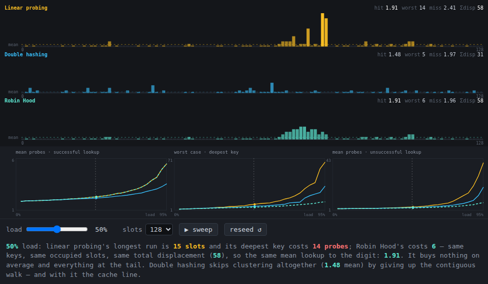
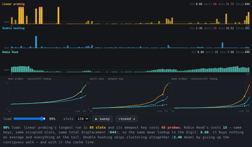
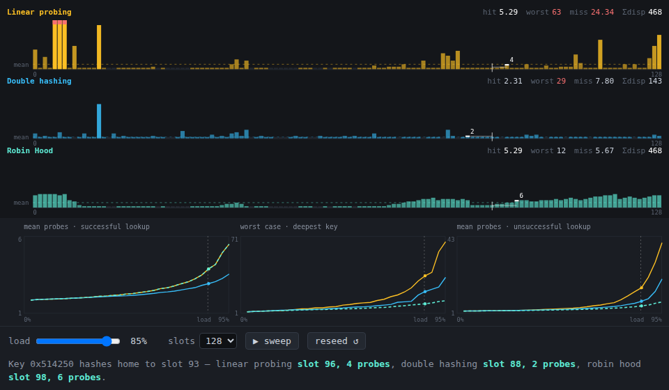
Three hash tables, one key stream, one hash function. Each table gets the same keys in the same order and differs only in where it puts them when the slot it wanted was taken. Every slot is drawn as a bar whose height is that key’s displacement — how far past its home slot it ended up — so a panel is a skyline of what lookups will cost.

Drag the load factor and the three skylines stop resembling each other:

• Linear probing grows staircases. A collision walks forward one slot at a time, so keys pile up behind each other and clusters merge into longer clusters, which catch more keys, which merge again. At 90% load on a 128-slot table the longest unbroken run is 89 slots and the deepest key costs 68 probes.
• Double hashing strides by h2(k) instead, so two keys that collide once almost never collide again. Its skyline is scattered spikes and its mean probe count barely moves: 2.40 where linear probing is at 6.60.
• Robin Hood walks forward exactly like linear probing, but when the key in hand is further from home than the slot’s current resident, it takes the slot and the richer key carries on. Same walk, different tenancy.

And here is the thing the picture is built to show. Robin Hood does not make the table faster on average. It cannot. At 90% load both linear panels report a mean of 6.60 probes and a total displacement of 644 — not close, identical, at every load factor and every seed. What changes is the shape: linear probing’s worst key costs 68 probes and Robin Hood’s costs 15. The bars are a redistribution, not a reduction.

Why the total can’t move

Cut the ring at any empty slot (open addressing always leaves one). Now look at a single cluster — a maximal run of occupied slots. Every key in that run is homed inside the run and sits at or after its home, so:

total displacement  =  Σ (slot it occupies)  −  Σ (slot it hashes to)

The second sum is fixed by the keys. The first is fixed too, because linear probing fills the same set of slots regardless of which key ends up in which — it never leaves a hole, so the occupied set depends only on the multiset of home positions. Both sums are settled before any policy gets a vote, and the total is their difference.

So a placement policy over a linear probe sequence has exactly one degree of freedom: who pays. First-come-first-served hands the whole bill to whoever arrives last, which is how you get a 68-probe key. Robin Hood spreads it evenly, which is why the panel is a hedge instead of a skyline. Averages are conserved; tails are a choice. (Verified rather than asserted: 1,000 random tables across five load factors, zero disagreements.)

Hover any bar to follow one key through all three tables at once — its home slot, where each policy put it, and what each lookup costs. It is worth finding a key that Robin Hood made worse: the flat tail is paid for by the keys that would otherwise have landed cheaply.

The column nobody looks at

miss is the mean probes for a key that isn’t in the table — the cost of every failed lookup, every “is this already here” check, every insert. It is the number that actually falls off a cliff. At 90% load linear probing needs 31.75 probes to conclude a key is absent, against Robin Hood’s 7.08 for the same keys in the same slots. Robin Hood gets to give up early: if the resident is closer to home than the searcher has walked, the searcher would have evicted it on the way in, so it cannot be further down the run. That early exit is free and it is most of the win.

Reuse

src/probe.js is a framework-free ES module — no DOM, no timers, no rendering:

• makeRng(seed) / makeKeys(count, m, rng) — deterministic keys carrying h1 (home) and h2 (an odd stride, so it is coprime with a power-of-two table).
• build(m, keys, strategy, count) — inserts the first count keys under 'linear' | 'double' | 'robin'; returns slots (key index per slot) and dist (the resident’s displacement), both Int32Array.
• placement(table) — the inverse view: slot and displacement per key.
• missProbes(table, key) — unsuccessful-search cost, including Robin Hood’s early exit.
• tableStats(table, queries) — mean/worst probes, total displacement, longest cluster, displacement histogram.
• curves(m, opts) — mean, worst and miss cost across load factors, averaged over independent key sets so the worst-case line is a trend and not noise.
• theory(alpha) — Knuth’s asymptotic expectations, for sanity checks.

Gotchas

• The hash is ideal here. h1 is uniform over the table, so every cluster in the linear panel is the placement policy’s own doing. Real clustering is this plus whatever your hash function is bad at.
• theory() is asymptotic and this table is small. At 128 slots and 95% load the formula predicts 10.5 probes; the actual table averages 5.5. The formulas assume m → ∞; don’t check a 128-slot measurement against them and conclude the code is broken.
• Probes are not cache misses. Double hashing wins every probe-count column and the demo counts probes, so it looks like a free lunch. It isn’t: linear probing’s next probe is usually in the cache line you already fetched, and double hashing’s is a fresh one. Which policy is actually fastest is a memory-system question this visualization does not answer.
• No deletion. Tombstones and Robin Hood’s backward-shift deletion are not modelled; every table here is insert-only. Adding deletion changes the displacement invariant, which is exactly why tombstoned tables degrade.
• One slot always stays empty (build caps at m - 1). An unsuccessful search in a completely full table has nothing to stop it.
• The demo bundles its own copy of probe.js (self-contained by contract); re-copy after editing src/.